Introduction

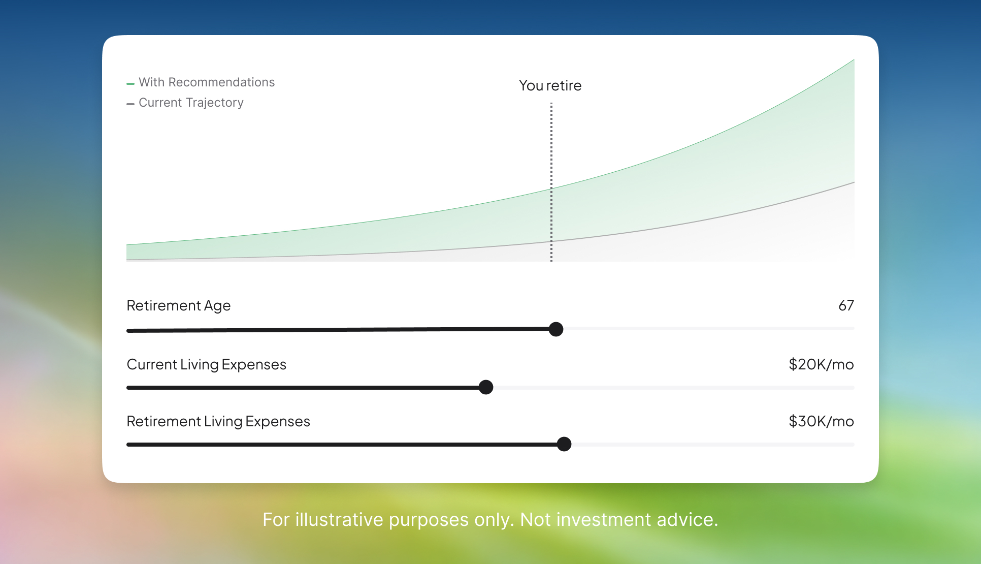
At Range, we use Monte Carlo simulations to calculate a household’s probability of success in achieving their retirement goals. Historically, these were run by planners before delivering a retirement plan. But members want to see the impact of life decisions on their retirement goals and iterate on their plans in real time. To support that, we built a live Retirement plan that immediately reflects any changes to a household’s information. Doing so required also speeding up the Monte Carlo simulation to deliver a delightful member experience.

By rewriting our simulation orchestration layer in Golang, we were able to reduce overall simulation time by ~39%, while maintaining the accuracy of our projections.

Background

Monte Carlo simulations are frequently used to estimate financial health for retirement planning. At Range, we run 1,000 trials to calculate probability of success for our members. Each trial runs from the current year through to the member’s end of plan (default is age 95). A trial is considered successful if the household has positive assets at the end of their plan after funding their goals and retirement expenses. We generally use an 80% probability-of-success target as one input in evaluating whether a household’s projected savings and spending plan appears sustainable.

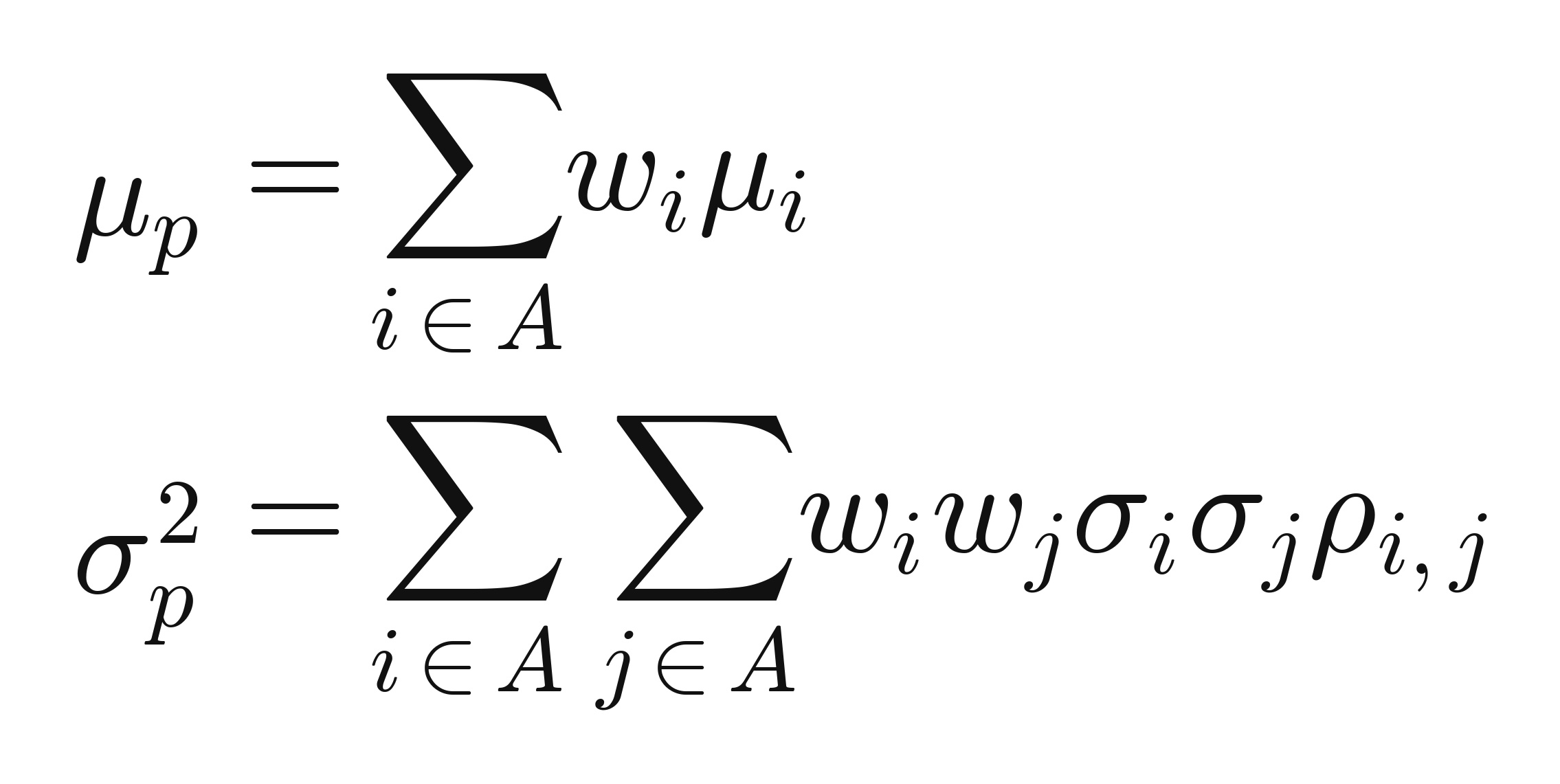
We compute the overall portfolio return μ_p and variance σ_p² across all investable assets for the household using a weighted sum of the portfolio allocations across all accounts of the household¹.

We then compute the investment return for a given year.

We estimate a household’s cash flow based on their actual and projected income and expenses. We then subtract any expenses related to life events such as purchasing a property or paying for college. Finally, we run a tax projection to calculate taxes such as capital gains, income, and property tax for the year and deduct those from the remaining cash flow.

Constrained by the remaining cash flow, we apply a savings waterfall strategy. We determine the recommended Roth/pre-tax split for contributions based on marginal tax rate for the household for the year. We maximize contributions to employer sponsored retirement accounts for the employer match and tax benefits, followed by IRAs and HSAs. Finally, any leftover cash flow is allocated to taxable brokerage accounts.

This process is run for every year starting from the current year through to the member’s end of plan (age 95). The overall simulation is repeated 1,000 times, and we display the probability of success and assets at the 25th, 50th, and 75th percentiles, giving a view of the household’s financial health across varying market conditions.

Existing Monte Carlo Simulation Architecture

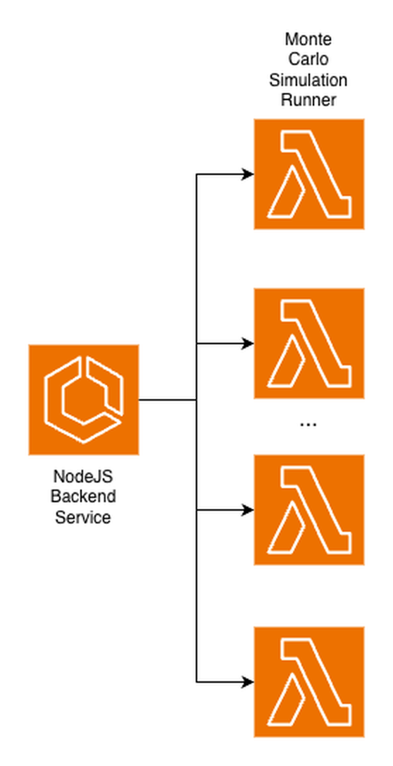
Our existing backend infrastructure consists of a NodeJS monolith running on ECS. The compute intensive nature of the Monte Carlo simulation made it a poor fit for running entirely on our backend NodeJS service. To offload that compute, our existing architecture used the backend service as an orchestrator and fanned out to 200 simulation runner Lambdas that ran 5 trials each.

This architecture had two problems. First, because the orchestration ran within our main backend service, the simulation competed with normal request traffic for a single event-loop thread. Second, Node scaled poorly as the number of concurrent runners grew. At 200 simulation runners, we saw ~500ms of invocation overhead before any trials ran, growing linearly with the number of runners.

Enter Golang

Our first step was to move the orchestrator out of the backend service and into a dedicated Lambda. Now each simulation ran in isolation, without impact from regular traffic or from other concurrent simulations.

To reduce latency, we tried increasing concurrency by dropping the trial batch size per runner from 5 to 1. Instead, latency got worse. The added invocations just piled more work onto the main thread.

Having traced the bottleneck to a single thread handling all invocations, we turned to Go, whose goroutines can parallelize them across multiple threads. Go wasn’t part of our stack, so normally this would have involved a significant learning curve and taken ~2 weeks to implement. With Claude, we could quickly test our hypothesis.

Before writing any code, we spent time in plan mode thinking through how to map the existing logic to Go. After writing the initial plan with Claude, we spun up review agents to catch anything we missed before implementing. To verify the port was functionally identical to the Node version, we ran the new orchestrator against every household in our member base and compared the probability of success. We fixed any regressions until the difference was 0% across all households. The entire loop of plan → implementation → verification took a little over a day. Finally, we benchmarked the Go orchestrator against NodeJS to measure the latency improvement.

Performance Benchmarks

We ran performance benchmarks using Go and Node for batch sizes of 1 and 5. The results are shown below.

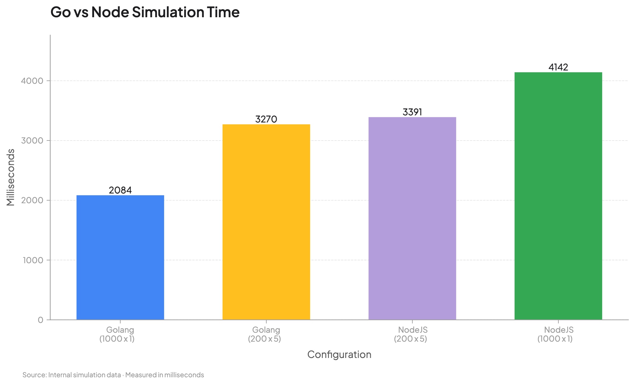
With a batch size of 5, Go showed no meaningful improvement over our existing configuration. However, reducing the batch size for both to 1, Go was 2x faster than Node. Increasing the fan-out led to higher latency with Node but lower with Go, confirming the single-thread bottleneck.

Overall, the Go implementation reduced simulation time by ~39%, giving us confidence to replace our existing architecture. This directly translated to faster page loads for members while still running a comprehensive simulation on the household’s most recent data.

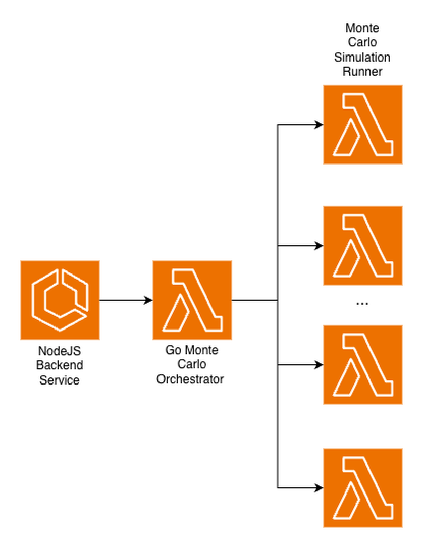
An additional benefit of the new architecture was a significant reduction in our regression test suite run time. Before each release, we run a Monte Carlo simulation for each household in our member base to measure the impact of a proposed change on their probability of success. The new orchestrator allowed us to run more simulations in parallel, reducing total run time from over 10 hours to under 2 hours. This let us go from testing a single change per day to several, so we can ship improvements and bug fixes much faster.

Takeaways

Below is a real-time view of the time required to run a complete Monte Carlo projection. Reducing the latency allowed us to build a better interactive experience for members without sacrificing accuracy of the projections.

If solving these kinds of problems and thinking outside the box is interesting to you, we’re hiring! See current openings here: https://www.range.com/public/careers

‍

Written in collaboration with Andrew Johnston and Scott Sadlo.

‍

^Footnotes

^{1. Where A is the set of allocations, wi is the percentage of assets for allocation i, and μi, σi, and ρij are respectively the rate of return for asset i, standard deviation for asset i, and correlation coefficient between assets i and j, provided by JP Morgan’s Long-Term Capital Market Assumptions, published annually.}